

Microeconomics
3D. (Step 2) Minimize TC for any given Q
a. Production Function (Photo by Slideshare)
- A production function is the relationship between
the quantity of inputs a firm uses, and the quantity output it produces.
- A fixed input is an input whose quantity is fixed
for a period and cannot be varied.
- A variable input is an input whose quantity the
firm can vary at any time.
- The long run is the time period in which all inputs
can be varied.
- The short run is the time period in which at least
one input is fixed.
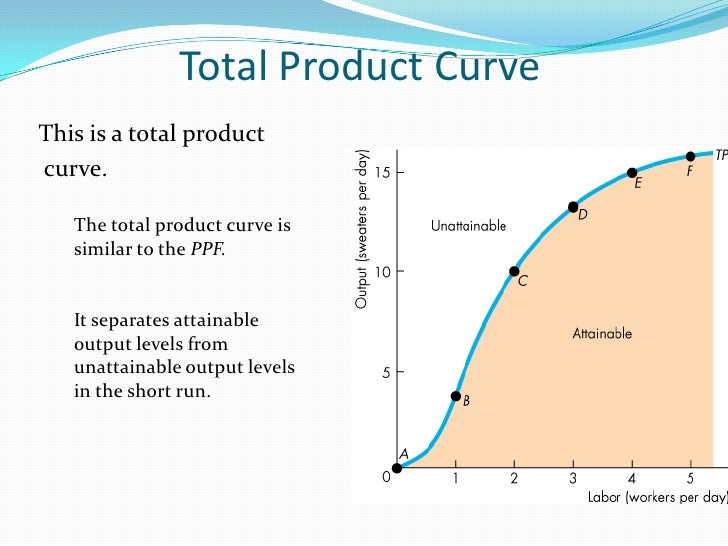
- The total product curve shows how the quantity of
output depends on the quantity variable input, for a given quantity of the
fixed output. The slope is equal to the marginal product of the variable
input.
- The marginal product of an input is the additional
quantity of output that is produced by using one more unit of that input.
- Marginal Product of Labor = Change in quantity of
output produce by one additional unit of labor
- Marginal Product of Labor = Change in Quantity of
Output / Change in Quantity of Labor
- In the short run, the fixed input cannot be varied.
- In the long run, all inputs are variable.
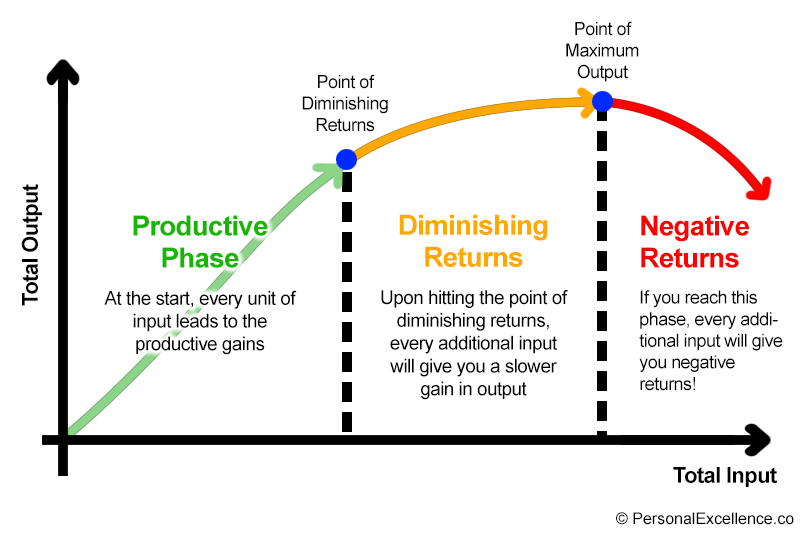
- There are diminishing returns to an input when an
increase in the quantity of that input, holding the levels of all other inputs
fixed, leads to a decline in the marginal product of that input.
- Diminishing returns to input might yield to a
downward-sloping marginal product curve and a total product curve that becomes
flatter as more output is produced.
- A fixed cost is a cost that does not depend on the
quantity of output produced. It is the cost of the fixed input.
- A variable cost is a cost that depends on the
quantity of output produced. It is the cost of the variable input.

- The total cost of producing a given quantity of
output is the sum of the fixed cost and the variable cost of producing that
quantity of output.
- Total Cost (TC) = Fixed Cost (FC) + Variable Cost (VC)
- The total cost curve shows how total cost depends
on the quantity of output.
- The total cost curve becomes more steeper as more
output is produced due to diminishing returns to the variable input.
b. Demand for Input (Factor)
- The value of the marginal product of a factor is
the value of the additional output generated by employing one more unit of that
factor.
- Value of the marginal product (VMP) = Price (P) x
Marginal Product (MP)
- Value of the marginal product of labor (VMP) =
Marginal cost of the producer (W) at the profit-maximizing level of employment.
-The price-taking firm’s optimal output rule: a
price-taking firm’s profit is maximized by producing the quantity of output at
which the marginal cost of the last unit produced is equal to the market price.
- A profit-maximizing price-taking producer employs
each factor of production up to the point at which the value of the marginal
product of the last unit of the factor employed is equal to that factor’s
price.
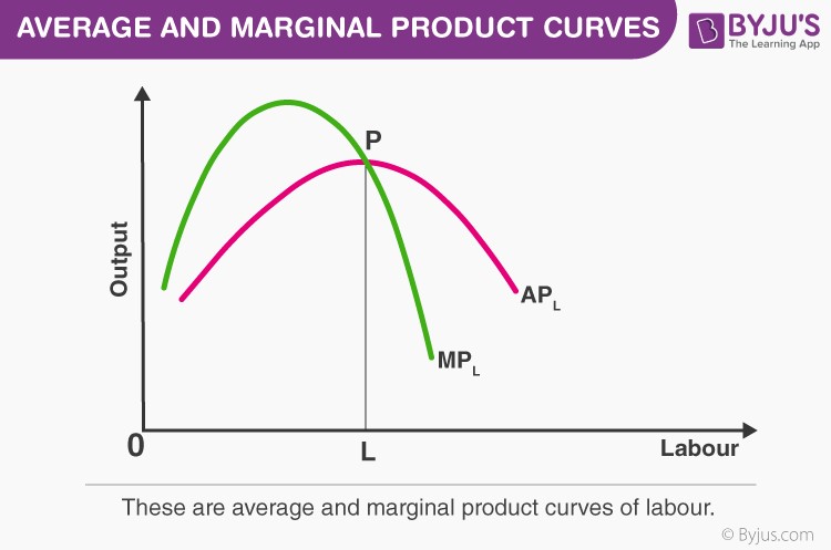
- The value of the
marginal product curve of a factor
shows how the value of the marginal product of that factor depends on the
quantity of the factor employed.
Shifts of the Factor Demand Curve
- Changes in price of output: if the price of the good that
is produced with a factor changes, so will the value of the marginal product of
the factor.
- Changes in supply of other factors: if the value of the
marginal product of labor curve shifts upward, at any given wage rate the
profit-maximizing level of employment rises.
- Changes in technology: improved technology can increase or
reduce the demand for a given factor of production.
Marginal-Productivity Rule:
VMP (input) = P (output) x MP (input)
Q (input) at P (input) = VMP (input)
VMP > P, increase Q
VMP < P, decrease Q
VMP = P, optimum level of output

- In a perfectly competitive market economy, the price of
the good multiplied by the marginal product of labor is equal to the value
of the marginal product of labor: VMPL = P x MPL.
- A profit-maximizing hires labor up to the point at which
the value of the marginal product of labor is equal to the wage rate: VMPL
= W.
- The value of the marginal product curve of labor
slopes downward due to diminishing returns to labor in production.
- The value of the marginal product curve is
therefore the individual price-taking producer’s demand curve for a factor.
- The market demand curve for labor is the horizontal sum of
all the individual demand curves of producers in that market. It shifts for
three reasons: changes in output, changes in the supply of other
factors, and technological progress.


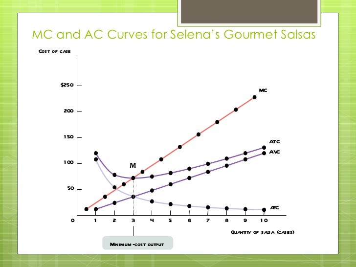
c. Cost Curve
Short Run Cost Curve
- Total Cost Curve: Total Costs = Fixed Cost + Variable Cost
(TC = FC + VC)
- The total cost curve shows how total cost depends
on the quantity of output. It becomes steeper as more output is produced due to
diminishing returns to the variable input
- Quantity INCREASES, Marginal Product DECREASES,
Value of Marginal Product DECREASES.
- Having determined the optimal quantity of output, we can
go back to the production function and find the optimal number of workers – it
is simply the number of workers needed to produce the optimal quantity of
output.
Average Cost Curve
- Average Total Cost = Average Fixed Cost + Average Variable
Cost (ATC = AFC + AVC)
- Average Total Cost = Total Cost (TC) / Quantity of Output
(Q)
- Average total cost (average cost) is the total cost
divided by quantity of output produced.
- When the U-shaped average total cost curve slopes
downward, the spreading effect dominates fixed cost is spread over more units
of output. (average fixed cost falls)
- When the U-shaped average total cost curve slopes
upward, the diminishing returns effect dominates: an additional unit of output
requires more variable inputs. (average variable cost rises)
- Average fixed cost = Fixed Cost (FC) / Quantity of Output
(Q)
- Average fixed cost is the fixed cost per unit of
output.
- Average variable cost = Variable Cost (VC) / Quantity of
Output (Q)
- Average variable cost is the variable cost per unit
of output.
Marginal Cost Curve
- The marginal cost of producing a good or service is
the additional cost incurred by producing one more unit of that good or
service.
- The marginal cost curve shows how the cost of
producing one more unit depends on the quantity that has already been produced.
- Production of a good or service has increasing marginal
cost when each additional unit costs more to produce than the previous one.
- Production of a good or service has constant marginal
cost when each addition unit costs the same to produce as the previous one.
- Production of a good or service has decreasing marginal
cost when each additional unit costs less to produce than the previous one.
Marginal Curve (MC), Marginal Cost = Marginal Variable
Cost (MC = MVC)
- The marginal benefit of a good or service is the
additional benefit derived from producing one more unit of that good or
service.
- Increasing marginal cost is reflected by an upward-sloping
marginal cost curve.
- Constant marginal cost is reflected by a horizontal
marginal cost curve.
- Decreasing marginal cost is reflected by a downward-sloping
marginal cost curve.
Marginal Cost Formula
- Marginal cost = Change in total cost generated by
one additional unit of output
- Marginal cost = Change in total cost / Change in
quantity of output
Marginal Cost Curves
- If marginal cost is above average total cost, average
total cost is rising.
- If marginal cost is below average total cost, average
total cost is falling.
- Increasing specialization initially leads to lower
marginal cost, but diminishing returns set in once the benefits from specialization
are exhausted and marginal cost rises.
- Marginal cost is equal to the slope of the total cost
curve.
- Diminishing returns cause the marginal cost curve to slope
upward.
- At low levels of output there are often increasing returns
to the variable input due to the benefits of specialization, making the
marginal cost curve “swoosh”-shaped: initially sloping downward before sloping
upward.
Total-Marginal Relationship
- Total cost increases whenever marginal cost is positive,
regardless of whether marginal cost is increasing or decreasing.
Marginal-Average Relationship
- Marginal cost slopes upward – the result of diminishing
returns that make an additional unit of output more costly to produce than the
one before.
- Average variable cost also slopes upward – again,
due to diminishing returns – but is flatter than the marginal cost curve. This is
because the higher cost of an additional unit of output is averaged across all units,
not just the additional units, in the average variable cost measure.
- Average fixed cost slopes downward because of the
spreading effect.
Minimum-Cost Output (Photo by SlideShare)
- The minimum-cost output is the quantity of output
at which average total cost is lowest – the bottom of the U-shaped average
total cost curve.
- At the minimum-cost output, average total cost =
marginal cost.
- At output less than the minimum-cost output, MC
< ATC, and ATC is falling.
- At output greater than the minimum-cost output, MC
> ATC, and ATC is rising.
Summary
Short Run
- Fixed cost (FC): cost that does not depend on the
quantity of output produced.
- Average fixed cost (AFC = FC / Q): fixed cost per
unit of output.
Short and Long Run
- Variable cost (VC): Cost that depends on the
quantity of output produced.
- Average variable cost (AVC = VC / Q): Variable cost
per unit of output.
- Total cost (TC = FC (short run) + VC): The sum of
fixed cost (short run) and variable cost.
- Average total cost (ATC = TC / Q): Total cost per
unit of output
- Marginal cost (MC = Change in TC / Change in Q):
The change in total cost generated by producing one more unit of output.
Long Run
- Long-run average total cost (LRATC): shows the relationship
between average total cost when fixed cost has been chosen to minimize average
total cost for each level of output.
- In the long run, a firm’s fixed cost becomes a variable it
can choose.
- As output increases, there are increasing returns to
scale if long-run ATC declines.
- As output increases, there are decreasing returns to
scale if long-run ATC increases.
- As output increase, there are constant returns to scale
if long-run ATC remains constant.
- Scale effects depend on the technology of production.